Image classification is a very large field of study, encompassing a wide variety of techniques – and with the popularity of deep learning, it is continuing to grow.

Image classification and image understanding are currently (and will continue to be) the most popular sub-field of computer vision for the next ten years. In the future, we’ll see companies like Google, Microsoft, Baidu, and others quickly acquire successful image understanding startup companies. We’ll see more and more consumer applications on our smartphones that can understand and interpret the contents of an image. Even wars will likely be fought using unmanned aircrafts that are automatically guided using computer vision algorithms.

Inside this chapter, I’ll provide a high-level overview of what image classification is, along with the many challenges an image classification algorithm has to overcome. We’ll also review the three different types of learning associated with image classification and machine learning.

Finally, we’ll wrap up this chapter by discussing the four steps of training a deep learning network for image classification and how this four step pipeline compares to the traditional, hand-engineered feature extraction pipeline

1. What Is Image Classification?

Image classification, at its very core, is the task of assigning a label to an image from a predefined set of categories.

Practically, this means that our task is to analyze an input image and return a label that categorizes the image. The label is always from a predefined set of possible categories. For example, let’s assume that our set of possible categories includes:

categories = {cat, dog, panda}

Then we present the following image (Figure 4.1) to our classification system:

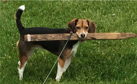
Our goal here is to take this input image and assign a label to it from our categories set – in this case, dog.

Our classification system could also assign multiple labels to the image via probabilities, such as dog: 95%; cat: 4%; panda: 1%.

More formally, given our input image of W × H pixels with three channels, Red, Green, and Blue, respectively, our goal is to take the W × H × 3 = N pixel image and figure out how to correctly classify the contents of the image.

1.1. A Note on Terminology

When performing machine learning and deep learning, we have a dataset we are trying to extract knowledge from. Each example/item in the dataset (whether it be image data, text data, audio data, etc.) is a data point. A dataset is therefore a collection of data points.

Our goal is to apply a machine learning and deep learning algorithms to discover underlying patterns in the dataset, enabling us to correctly classify data points that our algorithm has not encountered yet. Take the time now to familiarize yourself with this terminology:

1. In the context of image classification, our dataset is a collection of images.
2. Each image is, therefore, a data point.

I’ll be using the term image and data point interchangeably throughout the rest of this blog, so keep this in mind now.

1.2. The Semantic Gap

Given that all a computer sees is a big matrix of pixels, we arrive at the problem of the semantic gap. The semantic gap is the difference between how a human perceives the contents of an image versus how an image can be represented in a way a computer can understand the process.

How do we go about encoding all this information in a way that a computer can understand it? The answer is to apply feature extraction to quantify the contents of an image. Feature extraction is the process of taking an input image, applying an algorithm, and obtaining a feature vector (i.e., a list of numbers) that quantifies our image.

To accomplish this process, we may consider applying hand-engineered features such as HOG, LBPs, or other “traditional” approaches to image quantifying. Another method is to apply deep learning to automatically learn a set of features that can be used to quantify and ultimately label the contents of the image itself.

2. The Deep Learning Classification Pipeline

In this section we’ll review an important shift in mindset you need to take on when working with machine learning. From there I’ll review the four steps of building a deep learning-based image classifier as well as compare and contrast traditional feature-based machine learning versus end-to-end deep learning.

2.1. A Shift in Mindset

Unlike coding up an algorithm to compute the Fibonacci sequence or sort a list of numbers, it’s not intuitive or obvious how to create an algorithm to tell the difference between pictures of cats and dogs. Therefore, instead of trying to construct a rule-based system to describe what each category “looks like”, we can instead take a data driven approach by supplying examples of what each category looks like and then teach our algorithm to recognize the difference between the categories using these examples.

We call these examples our training dataset of labeled images, where each data point in our training dataset consists of:

1. An image
2. The label/category (i.e., dog, cat, panda, etc.) of the image Again, it’s important that each of these images have labels associated with them because our supervised learning algorithm will need to see these labels to “teach itself” how to recognize each category. Keeping this in mind, let’s go ahead and work through the four steps to constructing a deep learning model

   2.2. Step #1: Gather Your Dataset

   The first component of building a deep learning network is to gather our initial dataset. We need the images themselves as well as the labels associated with each image. These labels should come from a finite set of categories, such as: categories = dog, cat, panda.

Furthermore, the number of images for each category should be approximately uniform (i.e., the same number of examples per category). If we have twice the number of cat images than dog images, and five times the number of panda images than cat images, then our classifier will become naturally biased to overfitting into these heavily-represented categories.

Class imbalance is a common problem in machine learning and there exist a number of ways to overcome it. We’ll discuss some of these methods later in this book, but keep in mind the best method to avoid learning problems due to class imbalance is to simply avoid class imbalance entirely

2.3. Step #2: Split Your Dataset

Now that we have our initial dataset, we need to split it into two parts:

1. A training set
2. A testing set

A training set is used by our classifier to “learn” what each category looks like by making predictions on the input data and then correct itself when predictions are wrong. After the classifier has been trained, we can evaluate the performing on a testing set

It’s extremely important that the training set and testing set are independent of each other and do not overlap! If you use your testing set as part of your training data, then your classifier has an unfair advantage since it has already seen the testing examples before and “learned” from them. Instead, you must keep this testing set entirely separate from your training process and use it only to evaluate your network.

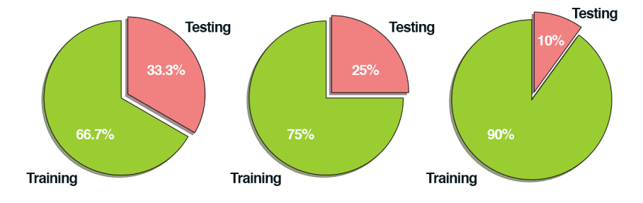
Common split sizes for training and testing sets include 66:6%33:3%, 75%=25%, and 90%=10%, respectively.

These data splits make sense, but what if you have parameters to tune? Neural networks have a number of knobs and levers (ex., learning rate, decay, regularization, etc.) that need to be tuned and dialed to obtain optimal performance. We’ll call these types of parameters hyperparameters, and it’s critical that they get set properly.

In practice, we need to test a bunch of these hyperparameters and identify the set of parameters that works the best. You might be tempted to use your testing data to tweak these values, but again, this is a major no-no! The test set is only used in evaluating the performance of your network.\

Instead, you should create a third data split called the validation set. This set of the data (normally) comes from the training data and is used as “fake test data” so we can tune our hyperparameters. Only after have we determined the hyperparameter values using the validation set do we move on to collecting final accuracy results in the testing data.

We normally allocate roughly 10-20% of the training data for validation. If splitting your data into chunks sounds complicated, it’s actually not. As we’ll see in our next chapter, it’s quite simple and can be accomplished with only a single line of code thanks to the scikit-learn library.

2.4. Step #3: Train Your Network

Given our training set of images, we can now train our network. The goal here is for our network to learn how to recognize each of the categories in our labeled data. When the model makes a mistake, it learns from this mistake and improves itself.

So, how does the actual “learning” work? In general, we apply a form of gradient descent, as discussed in after. The remainder of this blog is dedicated to demonstrating how to train neural networks from scratch, so we’ll defer a detailed discussion of the training process until then.

2.5. Step #4: Evaluate Your Network

Last, we need to evaluate our trained network. For each of the images in our testing set, we present them to the network and ask it to predict what it thinks the label of the image is. We then tabulate the predictions of the model for an image in the testing set.

Finally, these model predictions are compared to the ground-truth labels from our testing set. The ground-truth labels represent what the image category actually is. From there, we can compute the number of predictions our classifier got correct and compute aggregate reports such as precision, recall, and f-measure, which are used to quantify the performance of our network as a whole.

2.6. Feature-based Learning versus Deep Learning for Image Classification

In the traditional, feature-based approach to image classification, there is actually a step inserted between Step #2 and Step #3 – this step is feature extraction. During this phase, we apply handengineered algorithms such as HOG [32], LBPs [21], etc. to quantify the contents of an image based on a particular component of the image we want to encode (i.e., shape, color, texture). Given these features, we then proceed to train our classifier and evaluate it.

When building Convolutional Neural Networks, we can actually skip the feature extraction step. The reason for this is because CNNs are end-to-end models. We present the raw input data (pixels) to the network. The network then learns filters inside its hidden layers that can be used to discriminate amongst object classes. The output of the network is then a probability distribution over class labels.

One of the exciting aspects of using CNNs is that we no longer need to fuss over handengineered features – we can let our network learn the features instead. However, this tradeoff does come at a cost. Training CNNs can be a non-trivial process, so be prepared to spend considerable time familiarizing yourself with the experience and running many experiments to determine what does and does not work

2.7. What Happens When my Predictions Are Incorrect?

Inevitably, you will train a deep learning network on your training set, evaluate it on your test set (finding that it obtains high accuracy), and then apply it to images that are outside both your training and testing set – only to find that the network performs poorly.

This problem is called generalization, the ability for a network to generalize and correctly predict the class label of an image that does not exist as part of its training or testing data. The ability for a network to generalize is quite literally the most important aspect of deep learning research – if we can train networks that can generalize to outside datasets without retraining or fine-tuning, we’ll make great strides in machine learning, enabling networks to be re-used in a variety of domains. The ability of a network to generalize will be discussed many times in this blog, but I wanted to bring up the topic now since you will inevitably run into generalization issues, especially as you learn the ropes of deep learning.

Instead of becoming frustrated with your model not correctly classifying an image, consider the set of factors of variation mentioned above. Does your training dataset accurately reflect examples of these factors of variation? If not, you’ll need to gather more training data (and read the rest of this blog to learn other techniques to combat generalization)

3. Summary

Inside this chapter we learned what image classification is and why it’s such a challenging task for computers to perform well on (even though humans do it intuitively with seemingly no effort). Finally, we reviewed the four steps in the deep learning classification pipeline. These steps including gathering your dataset, splitting your data into training, testing, and validation steps, training your network, and finally evaluating your model. Unlike traditional feature-based approaches which require us to utilize hand-crafted algorithms to extract features from an image, image classification models, such as Convolutional Neural Networks, are end-to-end classifiers which internally learn features that can be used to discriminate amongst image classes.

4. References

• [1] Adrian Rosebrock, “Image Classification with Deep Learning and Python,” PyImageSearch, 2017. [Online]. Available: https://www.pyimagesearch.com/2017/08/21/ deeplearning -image-classification/. [Accessed: 01- Mar -2018].
• [2] ChatGPT Bot [Online]. Available: https://chatgpt.com/.