1. Pixels: The Building Blocks of Images

Before deep into Computer Vision, we first need to understand what an image is. We’ll start with the buildings blocks of an image – the pixel.

Pixels are the raw building blocks of an image. Every image consists of a set of pixels. There is no finer granularity (độ chi tiết tốt hơn) than the pixel.

Normally, a pixel is considered the “color” or the “intensity” (cường độ) of light that appears in a given place in our image. If we think of an image as a grid, each square contains a single pixel. For example, take a look at Figure 3.1.

The image in Figure 3.1 above has a resolution of 1.000×750, meaning that it is 1.000 pixels wide and 750 pixels tall. We can conceptualize an image as a (multidimensional) matrix. In this case, our matrix has 1.000 columns (the width) with 750 rows (the height). Overall, there are 1.000×750 = 750.000 total pixels in our image.

Most pixels are represented in two ways:

1. Grayscale/single channel
2. Color

In a grayscale image, each pixel is a scalar value between 0 and 255, where zero corresponds to “black” and 255 being “white”. Values between 0 and 255 are varying shades of gray, where values closer to 0 are darker and values closer to 255 are lighter.

Color pixels; however, are normally represented in the RGB color space (other color spaces do exist, but are outside the scope of my blog and not relevant for deep learning).

Pixels in the RGB color space are no longer a scalar value like in a grayscale/single channel image – instead, the pixels are represented by a list of three values: one value for the Red component, one for Green, and another for Blue. To define a color in the RGB color model, all we need to do is define the amount of Red, Green, and Blue contained in a single pixel.

Each Red, Green, and Blue channel can have values defined in the range [0;255] for a total of 256 “shades”, where 0 indicates no representation and 255 demonstrates full representation. Given that the pixel value only needs to be in the range [0;255], we normally use 8-bit unsigned integers to represent the intensity.

As we’ll see once we build our first neural network, we’ll often preprocess our image by performing mean subtraction or scaling, which will require us to convert the image to a floating point data type. Keep this point in mind as the data types used by libraries loading images from disk (such as OpenCV) will often need to be converted before we apply learning algorithms to the images directly.

Given our three Red, Green, and Blue values, we can combine them into an RGB tuple in the form (red, green, blue). This tuple represents a given color in the RGB color space. The RGB color space is an example of an additive color space: the more of each color is added, the brighter the pixel becomes and closer to white. We can visualize the RGB color space in Figure 3.3 (left). As you can see, adding red and green leads to yellow. Adding red and blue yields pink. And adding all three red, green, and blue together, we create white.

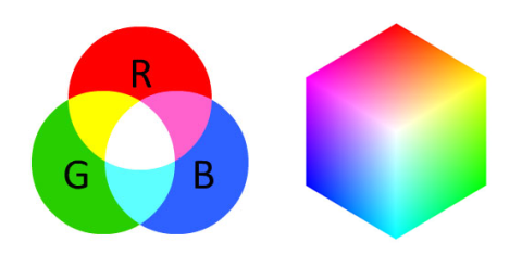
To make this example more concrete, let’s again consider the color “white” – we would fill each of the red, green, and blue buckets up completely, like this: (255, 255, 255). Then, to create the color black, we would empty each of the buckets out (0, 0, 0), as black is the absence of color. To create a pure red color, we would fill up the red bucket (and only the red bucket) completely: (255, 0, 0).

The RGB color space is also commonly visualized as a cube (Figure 3.3, right) Since an RGB color is defined as a 3-valued tuple, which each value in the range [0;255] we can thus think of the cube containing 256×256×256 = 16;777;216 possible colors, depending on how much Red, Green, and Blue are placed into each bucket.

The primary drawbacks of the RGB color space include:

• Its additive nature makes it a bit unintuitive for humans to easily define shades of color without using a “color picker” tool.
• It doesn’t mimic how humans perceive color. Despite these drawbacks, nearly all images you’ll work with will be represented (at least initially) in the RGB color space.

  1.1. Forming an Image from Channels

As we now know, an RGB image is represented by three values, one for each of the Red, Green, and Blue components, respectively. We can conceptualize an RGB image as consisting of three independent matrices of width W and height H, one for each of the RGB components, as shown in Figure 3.5. We can combine these three matrices to obtain a multi-dimensional array with shape W × H × D where D is the depth or number of channels (for the RGB color space, D=3):

Keep in mind that the depth of an image is very different than the depth of a neural network – this point will become clear when we start training our own Convolutional Neural Networks. However, for the time being simply understand that the vast majority of the images you’ll be working with are:

• Represented in the RGB color space by three channels, each channel in the range [0;255]. A given pixel in an RGB image is a list of three integers: one value for Red, second for Green, and a final value for Blue.
• Programmatically defined as a 3D NumPy multidimensional arrays with a width, height, and depth.

  2. Image Coordinate System

  As mentioned in Figure 3.1 earlier in this chapter, an image is represented as a grid of pixels. To make this point more clear, imagine our grid as a piece of graph paper. Using this graph paper, the origin point (0;0) corresponds to the upper-left corner of the image. As we move down and to the right, both the x and y values increase.

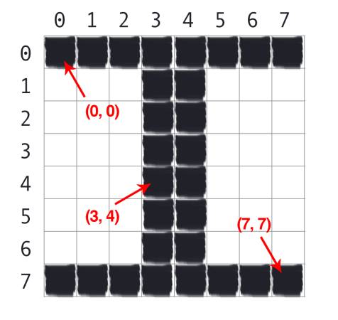
Figure 3.4 provides a visual representation of this “graph paper” representation. Here we have the letter “I” on a piece of our graph paper. We see that this is an 8 × 8 grid with a total of 64 pixels.

It’s important to note that we are counting from zero rather than one. The Python language is zero indexed, meaning that we always start counting from zero. Keep this in mind as you’ll avoid a lot of confusion later on (especially if you’re coming from a MATLAB environment).

As an example of zero-indexing, consider the pixel 4 columns to the right and 5 rows down is indexed by the point (3;4), again keeping in mind that we are counting from zero rather than one.

2.1. Image as Numpy Arrays

Image processing libraries such as OpenCV and scikit-image represent RGB images as multidimensional NumPy arrays with shape (height, width, depth). Readers who are using image processing libraries for the first time are often confused by this representation – why does the height come before the width when we normally think of an image in terms of width first then height?

The answer is due to matrix notation.

When defining the dimensions of matrix, we always write it as rows x columns. The number of rows in an image is its height whereas the number of columns is the image’s width. The depth will still remain the depth.

Therefore, while it may be slightly confusing to see the .shape of a NumPy array represented as (height, width, depth), this representation actually makes intuitive sense when considering how a matrix is constructed and annotated.

For example, let’s take a look at the OpenCV library and the cv2.imread function used to load an image from disk and display its dimensions:

import cv2
image = cv2.imread("example.png")
print(image.shape)
cv2.imshow("Image", image)
cv2.waitKey(0)

Here we load an image named example.png from disk and display it to our screen, as the screenshot from Figure 3.7 demonstrates. My terminal output follows:

$ python load_display.py
(248, 300, 3) 

This image has a width of 300 pixels (the number of columns), a height of 248 pixels (the number of rows), and a depth of 3 (the number of channels). To access an individual pixel value from our image we use simple NumPy array indexing:

(b, g, r) = image[20, 100] # accesses pixel at x=100, y=20
(b, g, r) = image[75, 25] # accesses pixel at x=25, y=75
(b, g, r) = image[90, 85] # accesses pixel at x=85, y=90

Again, notice how the y value is passed in before the x value – this syntax may feel uncomfortable at first, but it is consistent with how we access values in a matrix: first we specify the row number then the column number. From there, we are given a tuple representing the Red, Green, and Blue components of the image.

2.2. RGB and BGR Ordering

It’s important to note that OpenCV stores RGB channels in reverse order. While we normally think in terms of Red, Green, and Blue, OpenCV actually stores the pixel values in Blue, Green, Red order.

Why does OpenCV do this?The answer is simply historical reasons. Early developers of the OpenCV library chose the BGR color format because the BGR ordering was popular among camera manufacturers and other software developers at the time [41].

Simply put – this BGR ordering was made for historical reasons and a choice that we now have to live with. It’s a small caveat, but an important one to keep in mind when working with OpenCV.

3. Scaling and Resizing

Scaling, or simply resizing, is the process of increasing or decreasing the size of an image in terms of width and height. When resizing an image, it’s important to keep in mind the aspect ratio, which is the ratio of the width to the height of the image. Ignoring the aspect ratio can lead to images that look compressed and distorted, as in Figure 3.5.

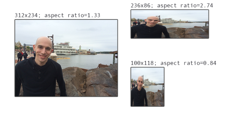
On the left, we have the original image. And on the top and bottom, we have two images that have been distorted by not preserving the aspect ratio. The end result is that these images are distorted, crunched, and squished. To prevent this behavior, we simply scale the width and height of an image by equal amounts when resizing an image.

From a strictly aesthetic point of view, you almost always want to ensure the aspect ratio of the image is maintained when resizing an image – but this guideline isn’t always the case for deep learning. Most neural networks and Convolutional Neural Networks applied to the task of image classification assume a fixed size input, meaning that the dimensions of all images you pass through the network must be the same. Common choices for width and height image sizes inputted to Convolutional Neural Networks include 32×32, 64×64, 224×224, 227×227, 256×256, and 299×299

Let’s assume we are designing a network that will need to classify 224×224 images; however, our dataset consists of images that are 312×234, 800×600, and 770×300, among other image sizes – how are we supposed to preprocess these images? Do we simply ignore the aspect ratio and deal with the distortion. Or do we devise another scheme to resize the image, such as resizing the image along its shortest dimension and then taking the center crop.

The aspect ratio of the image has been maintained, but at the expense of cropping out part of the image. This could be especially detrimental to our image classification system if we accidentally crop part or all of the object we wish to identify.

Which method is best? In short, it depends. For some datasets you can simply ignore the aspect ratio and squish, distort, and compress your images prior to feeding them through your network. On other datasets, it’s advantageous to preprocess them further by resizing along the shortest dimension and then cropping the center.

4. Summary

This chapter reviewed the fundamental building blocks of an image – the pixel. We learned that grayscale/single channel images are represented by a single scalar, the intensity/brightness of the pixel. The most common color space is the RGB color space where each pixel in an image is represented by a 3-tuple: one for each of the Red, Green, and Blue components, respectively.

We also learned that computer vision and image processing libraries in the Python programming language leverage the powerful NumPy numerical processing library and thus represent images as multi-dimensional NumPy arrays. These arrays have the shape (height, width, depth).

The height is specified first because the height is the number of rows in the matrix. The width comes next, as it is the number of columns in the matrix. Finally, the depth controls the number of channels in the image. In the RGB color space, the depth is fixed at depth=3.

Finally, we wrapped up this chapter by reviewing the aspect ratio of an image and the role it will play when we resize images as inputs to our neural networks and Convolutional Neural Networks.